
By: Clinton Brownley, Lead Data Scientist
At Tala, we want to continuously improve our product and user experience. So, to learn whether the changes we make are beneficial, we run experiments. By establishing short-term proxy metrics of long-term value outcomes, we are now able to gain insights more quickly, expedite the experiment process, and make informed decisions more quickly to unlock value to our customers.
We originally deemed naive predictive machine learning models to be poorly suited to the job, as treatment effect estimates gleaned from linear coefficients or feature sensitivity analysis are likely to be biased. We were excited to discover that a statistical modeling technique called the surrogate index addresses this problem head-on. The surrogate index combines early read metrics to estimate long-term treatment effects in a causally sound way more rapidly and, to our surprise, at times more precisely than would be available from a full-duration long-term experiment.
We reviewed the paper’s replication code and identified a couple of challenges: (1) it was written in Stata (our team writes Python and R code) and (2) it demonstrated the methodology using ordinary least squares (OLS) only, whereas the paper acknowledged that more flexible models might perform better. We overcame both of these challenges by implementing the methodology in Python and extending it with more flexible models.
Understanding and implementing the surrogate index
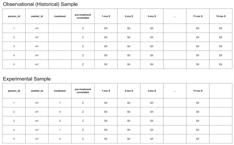
The surrogate index methodology involves using two datasets, one historical observational and another from an experiment, and has three modeling steps. The two datasets are similar, but the differences between them are crucial.
Historical observational dataset
The historical observational dataset includes the long-term outcome of interest and early measures of the long-term outcome (aka short-term proxies). It may also include additional predictor variables. Notably, it doesn’t include a treatment group indicator because the data are not from an experiment. For example, if the long-term outcome is the total amount of money repaid minus the total amount of money loaned (aka credit margin) one year after a loan was disbursed to a borrower, then early measures of this outcome might be monthly values of this quantity at one month after loan disbursement, two months after loan disbursement, and so on up to the value at eleven months after loan disbursement. So, for this example, the historical observational dataset would contain the twelve monthly values of credit margin for a set of loans disbursed well before the period of experimentation.
Experimental dataset
The dataset from an experiment includes a treatment group indicator and early measures of the long-term outcome. And like the historical observational dataset, it may also include additional predictor variables. It doesn’t include the long-term outcome because this is the value we don’t want to wait to observe and measure. So, for this example, the experimental dataset would contain a treatment group indicator and the early measures of the long-term outcome for a set of loans disbursed during the period of experimentation.
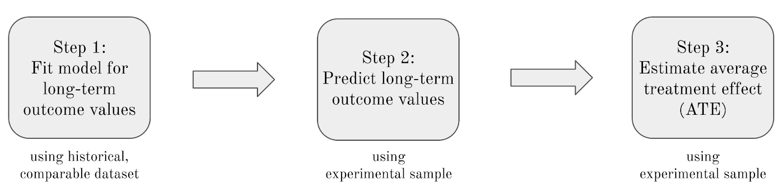
Three modeling steps
The surrogate index modeling technique involves three steps:
Step 1: Using the historical observational dataset, regress the long-term outcome on one or more short-term predictors and any additional pre-treatment predictors.
Step 2: Using the experimental dataset and the model from Step 1, pass the predictor variables in the experimental dataset (the same predictors used in Step 1) through the model from Step 1 and predict long-term outcome values for the records in the experimental dataset.
Step 3: Using the experimental dataset, regress the predicted long-term outcome values on the treatment group indicator to estimate the average treatment effect (ATE) of the experimental treatment on the long-term outcome.
Identifying the smallest sufficient set of surrogates
One goal of the surrogate index modeling technique is to identify the fewest short-term predictors needed to reliably estimate the average treatment effect because doing so can deliver a more precise estimate. Therefore, the technique is iterative, at least at the beginning, when determining the number of short-term predictors to include in the models.
For example, given the historical observational dataset described above, with its twelve monthly values of credit margin and no additional predictors, a first model for Step 1 could involve regressing the month-12 credit margin on the month-1 credit margin only. Next, for Step 2, one would pass the month-1 credit margin values in the experiment dataset through the model from Step 1 and predict long-term outcome values for the records in the experiment dataset. Finally, for Step 3, one would regress the predicted long-term outcome values on the treatment group indicator to estimate the treatment’s long-term ATE.
To determine the number of short-term predictors to include in the models, a second model for Step 1 could involve regressing the month-12 credit margin on both the month-1 and month-2 credit margins. In Step 2, one would pass the month-1 and month-2 credit margin values through the model and predict long-term outcome values for the records in the experiment dataset. Finally, for Step 3, one would regress the predicted long-term outcome values on the treatment group indicator to estimate the treatment’s long-term ATE.
This iterative process of constructing models with more and more short-term predictors would continue until the model in Step 1 contained all of the short-term predictors preceding the long-term outcome. In our example, this expanded model in Step 1 would regress the month-12 credit margin on eleven predictors: from month-1 to the month-11 credit margin.
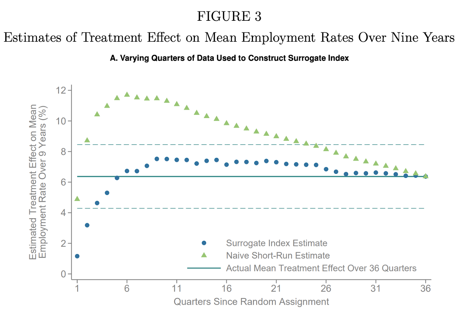
By evaluating this technique using a historical experiment where the long-term ATE has been measured, one can compare each of the eleven estimated ATEs to the actual, observed long-term ATE. One can then see which model estimates are similar to the observed ATE. According to the authors of the paper, the model with the fewest predictors that still recovers the observed ATE is preferred because “by identifying suitable surrogates…one can strip out the residual variation arising from downstream factors that create noise” thereby resulting in a more precise estimate. Figure 3 from the paper illustrates this iterative process; varying the number of short-term predictors included in the model identifies the model with the fewest predictors that still recovers the observed ATE.
Internal evaluation and validation
We were excited to discover a published technique that purported to solve our problem. However, before using it in live experiments that would influence our lending and repayment strategies and product features, we decided to validate it with our historical experiments.
These validation analyses allowed us both to evaluate the performance of models that are more flexible than OLS and to build the modeling technique in Metaflow, a Python library that makes it straightforward to develop, deploy, and operate various kinds of data-intensive applications.
To validate the technique, we evaluated it across a broad range of experiments and model types:
- We built many types of models, including Elasticnet (Enet), Generalized Additive Models (GAM), Random Forest (RF), Gradient-Boosted Trees (GBM), and Bayesian Additive Regression Trees (BART), and evaluated their performance with and without additional predictors.
- We evaluated its performance with historical experiments spanning across lending and repayment strategies, product features, and countries.
ATE estimates are unbiased
All of our validation analyses recovered the long-term ATEs we had observed in our historical experiments. That is, our estimated long-term ATEs were aligned with the actual ATEs, and our estimates’ bootstrapped 95% confidence intervals contained the actual ATEs. These results gave us and our business partners confidence in the technique, which paved the way for conversations about using it in future experiments.
ATE estimates are at times higher precision
Moreover, we observed the increase in the precision of the average treatment effects estimates that the authors discussed in their paper. The authors noted that the surrogate index “yields a substantial increase in precision…a 35% reduction in the standard error of the estimate” (in their application).
The authors explain this result can occur because “the surrogacy assumption brings additional information to bear on the problem – namely that any variation in the long-term outcome conditional on surrogates is orthogonal to treatment and hence is simply noise that increases the residual variance of the outcome and reduces precision.” So, “by identifying suitable surrogates…one can strip out the residual variation arising from downstream factors that create noise.” Therefore, “surrogates purge the most noise when the residual variances in treatment and the long-term outcome given surrogates are high, thereby yielding larger efficiency gains.”
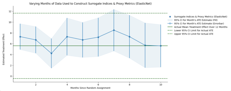
As shown in the above plot, the 95% confidence interval for the observed average treatment effect on our long-term outcome of interest (i.e., the green dotted lines) ranged from approximately 0 to 12. Whereas, the 95% confidence interval for the 1-month surrogate index estimate of the ATE (i.e., the leftmost blue vertical lines) ranged from approximately 5 to 10. That is, in our application, like in the authors’, the surrogate index yielded a substantial increase in precision — in our case, a 58% reduction in the width of the confidence interval. We observed similar increases in precision across our remaining validation analyses. As the authors pointed out, “the results imply that it is optimal to use the smallest set of surrogates that satisfy the surrogacy assumption to maximize efficiency.”
Succeeding with shorter, reliable, reproducible experiments
We have learned a lot by extending and validating the technique with our historical experiments, particularly the benefits of collaborating with business partners from the beginning, using flexible models, and building the technique in an infrastructure that makes it easy to develop, deploy, and operate.
First, by collaborating with our business partners to select the historical experiments, define the key variables and time frames, and review the results, we ensured our business partners were invested in the validation effort, understood the analyses, and were equally excited about the favorable results. Second, by extending the technique with flexible models and additional predictors, and comparing these models to OLS models with fewer variables, we were able to identify models we are confident will provide reliable estimates of long-term ATEs in future experiments. Third, by building the technique in a robust infrastructure, we have reliably reproduced results, generalized the technique across countries, experiments, and long-term outcomes, and enabled our partners to use it quickly, easily, and appropriately.
We have realized many benefits from validating and implementing the technique for internal experimentation. By building the technique in a robust infrastructure, we have enhanced and standardized this methodology. Now, analyses of experiment results are consistently reliable, reproducible, and of high quality. We are just coming out of the implementation and validation exercise. Now, with our validated approach to estimate these long-term ATEs more rapidly and reliably, we’re excited for the next phase: using them in our live experiments.